Sonic Liquidations: Unpriced Orderflow on Public Display
A DeFi trading case study on turning a concentrated Sonic lending-market anomaly into a levered carry trade, liquidation-path model, automated unwind, and event-driven short—and the governed endgame now forming.
This case study covers two connected trades. An anomalous Silo USDC yield led me to a concentrated S-backed borrower; I earned 21.79% net over 24 days while monitoring its solvency, automated my exit as compounding debt made the market increasingly fragile, and modeled the liquidation’s likely market impact. After refinancing temporarily removed the catalyst and falling S later restored it, I shorted S on Hyperliquid and earned 8.67% net on opening notional over 31h 55m.
The APY Anomaly
I regularly scan Silo because its smaller isolated markets often create mispriced, usually short-lived lending opportunities. In late April, its S/USDC market stood out: the interface showed USDC suppliers earning roughly 48.6%.
Curious about the headline rate, I compared the market with Aave and investigated why USDC liquidity was being priced so differently across the two venues. Around discovery, Silo also showed approximately 57% USDC borrow cost, with a 75% max LTV and 80% liquidation threshold. The loop I ultimately built borrowed S from Silo, supplied it through Aave, borrowed USDC against that collateral, and deposited the USDC back into Silo.
The rate discrepancy was the starting point, not the entry signal. The borrower’s health factor needed enough room for a short holding period, the net loop spread needed to remain positive after both borrowing legs, and observed deposit flow needed to support an incremental exit. At the loop’s May 1 start, the 1.37 health factor represented roughly 27% static collateral-value headroom before liquidation. That was meaningful, but not enough to make the position passive.
Withdrawal liquidity was a flow rather than a guaranteed balance. I had repeatedly seen new USDC arrive in roughly $25k to $50k clips, so the exit plan was to unwind into those deposits instead of assuming the entire position could leave at once. I monitored utilization, the borrower’s health factor, and incoming liquidity throughout the trade.
By May 1, when the analyzed loop began, utilization had pushed the displayed Silo rates to roughly 225% supply APY and 265% borrow APY. The position ran 1.54x time-weighted average leverage against net USDC equity, peaking at a modeled 1.83x.
Those interface APYs are approximate historical readings, not the basis of the performance calculation. Realized returns were reconstructed separately from block-bounded Silo and Aave deposit, withdrawal, borrow, and repayment events.
Over 24 days, unlevered Silo supply returned 10.51%. The loop returned 21.82% after Aave USDC borrowing costs and 21.79% after also marking the S borrow cost. The leverage added 11.32 percentage points and produced 2.08x the baseline period return.
Why The Yield Looked Wrong
The yield was not broad-based. It was being driven by the primary borrower, 0x8d4d19405ba352e4767681c28936fc0a9a8c8dfe, whose wallet showed no meaningful activity after a three-day collateral top-up ending February 1.
The loan was already more than a year old when I found it. The borrower opened it on February 15, 2025 by depositing 5,000,000 S ($2.58m) and borrowing $1.16m USDC four minutes later, at a 1.78 health factor. Later top-ups took the collateral to approximately 70m S by February 2026, including 30m S added after health factor had reached 1.01 on January 30.
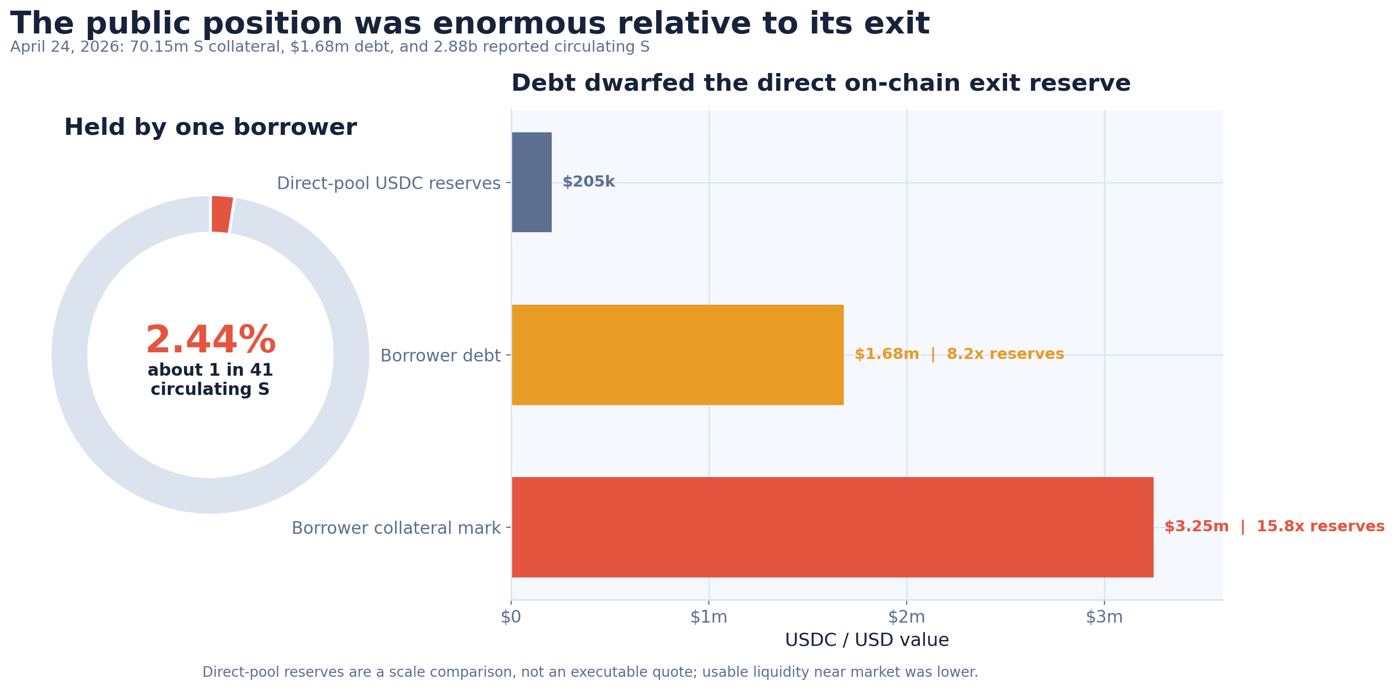
By April 24, the account held 70,154,068 S: 2.44% of the 2.88b reported circulating supply, or roughly one token in every 41. Its $1.68m debt was 8.2x the approximately $205k of USDC reserves I could reconstruct across direct wS/USDC pools. Marking the collateral at the public $0.0463 spot price put it at $3.25m, or 15.8x those reserves.
The Liquidity Gut Check
The direct-pool reserve comparison was only the first gut check. I also sampled executable routes rather than relying on market cap or headline daily volume. During the May research, my contemporaneous checks looked like this:
| Capacity check | Observation | $427,200 candidate clip |
|---|---|---|
| Direct wS/USDC pool reserves | Approximately $205k USDC | 2.1x the reserve balance |
| LlamaSwap S-to-USDC quotes | Slippage became economically prohibitive beyond roughly $600k of S input | 71% of the largest still-viable quoted sale |
| Binance S/USDT bid depth within 2% | Approximately $170k | 2.5x the visible near-market bids |
Those figures were not three independent pools of liquidity that could simply be added together. LlamaSwap already aggregated multiple on-chain routes, while arbitrageurs closing a DEX/CEX gap would buy discounted S on-chain and sell into the same Binance bids. The approximately $600k LlamaSwap ceiling also did not mean a $600k sale would clear cleanly; it marked the region where slippage began consuming the liquidation bonus and making a flash-loan liquidation uneconomic.
At $0.048 per S, the candidate first clip was 8,900,000 S, or $427,200. That was already 2.5x Binance’s visible 2% bid depth. Even if only part of the DEX dislocation reached Binance, exhausting that depth made an immediate low-single-digit repricing a central scenario rather than a remote tail. Holding debt and liquidation parameters fixed, a further 3% fall in S would also reduce an S-backed account’s health factor by approximately 3%, potentially pushing nearby borrowers toward eligibility. Partial liquidation changes both debt and collateral, so this was a sensitivity, not a forecast of the next clip.
That was the moment the yield anomaly became a forced-flow trade: a plausible first liquidation was already larger than the market’s clean exit capacity, and its own price impact could help create the next liquidation.
Was Anyone Else Watching?
I then tried to determine whether the overhang was already crowded. Searches for the address and market mostly surfaced explorer pages and generic yield listings, not analysis connecting the debt path to the liquidation overhang. The account had roughly eight DeBank followers when I checked; I reviewed them manually and they all appeared to be other depositors in the Silo market. None showed visible evidence of trading perps or positioning for the same directional short.
This was a small, non-random sample. DeBank cannot see CEX activity, alternate wallets, or anyone watching the position without following it, so it did not prove that nobody else had noticed. What it did suggest was a split: the people visibly in the lending market were there for the yield, and the directional traders I followed were not talking about the lending balance sheet that would eventually generate the forced flow.
The apparent edge was not private information. It was connecting a public lending balance sheet to the thin spot and perp markets that would eventually have to absorb its forced flow.
Historical archive calls make the full timeline and subsequent deterioration visible:
| Date and state | Venue | Collateral | Debt value | Health factor |
|---|---|---|---|---|
| Feb 15, 2025, position opened | Silo | 5,000,000 S / $2.58m | $1.16m | 1.78 |
| Apr 1, 2026, historical baseline | Silo | 70,150,000 S / $2.87m | $1.55m | 1.48 |
| May 1, 2026, loop opened | Silo | 70,160,000 S / $3.03m | $1.77m | 1.37 |
| May 22, 2026, before refinancing | Silo | 70,160,000 S / $3.23m | $2.08m | 1.24 |
| May 22, 2026, after refinancing | Silo residual | 17,160,000 S / $790,773 | $454,608 | 1.39 |
| May 22, 2026, after refinancing | Aave | 72,080,000 S-eq / $3.32m | $2.01m | 1.15 |
| Jun 23, 2026, first short fill | Aave | 94,170,000 S-eq / $2.30m | $1.53m | 1.05 |
| Jun 23, 2026, after first liquidation clip | Aave | 94,160,000 S-eq / $2.18m | $1.53m | 0.99 |
From April 1 to the first refinancing transaction, S collateral quantity remained almost flat and its oracle value actually increased 12.8%. Debt nevertheless grew 34.7%, taking the derived Silo health factor from 1.48 to 1.24. Interest-rate compounding, rather than an initial S selloff, did the early damage.
The same utilization spike paying me was steadily making the market’s largest borrower less solvent.
This was the condition the entry plan was designed to catch. The trade began with enough solvency and exit-liquidity headroom to justify the carry; as both narrowed, the correct response changed from harvesting yield to engineering the unwind.
Historical snapshot methodology and block provenance
The opening row is reconstructed from the borrower’s 5,000,000 S deposit and $1,160,000 USDC borrow at Sonic blocks 8022952 and 8023313. The state values shown are end-of-block reads after the borrow. The April 1 row predates discovery and is included as an earlier historical baseline. I found the opportunity in late April; the table does not claim an exact discovery-day snapshot.
The supply comparison uses CoinMarketCap’s April 24 snapshot: 2.88b S circulating, 3.22b S total supply, and a $0.0463 spot price. At Sonic block 68546468, the Silo position held 70,154,068 S and owed $1.68m. Historical USDC balanceOf calls at the same block sum approximately $205k held by the direct wS/USDC pools I could reconstruct. This is a reserve comparison, not an executable quote: indirect routes are excluded, and withdrawing the full reserve would require extreme slippage, so immediately executable liquidity near the prevailing price was lower.
The Silo rows and scale comparison use historical eth_call state at Sonic blocks 8023313, 66410980, 68546468, 69312914, 71207140, and 71209713. Collateral and debt shares were converted to assets with the relevant Silo accounting views. Collateral values use the market’s historical solvency-oracle quote, and health factor is derived from the 80% liquidation threshold:
health factor = collateral value * liquidation threshold / debt valueThe Aave rows use getUserAccountData at blocks 71209713 (after refinancing), 74513951, and 74537367. Block 74513951 is one second before the reconstructed short’s first fill; 74537367 is two blocks after the first Aave clip and one block before the next two clips. Collateral in those rows is also shown as S-equivalent (S-eq): the wS aToken balance plus the stS aToken balance converted at Beets’ stS-to-S exchange rate at the same block. The end-of-block health factor immediately before the burst was 1.03; the eligibility-changing state update occurred inside the first liquidation block, so an eth_call at the previous block cannot show the exact pre-transaction breach.
These are protocol position snapshots, not wallet-portfolio estimates. After refinancing, the exposure was split across accounts and protocols, so the Silo and Aave rows are reported separately rather than presented as a complete aggregate.
Model, Then Exit
As May progressed and the borrower’s health factor deteriorated, the relevant question was no longer the quoted APY. It was how much S would need to be sold, through which venues, and whether the resulting price impact could trigger further liquidations. I joined lending state, liquidation constraints, DEX quote curves, CEX bids, secondary borrowing, and Hyperliquid capacity into one path-dependent model.
The initial May model formalized the clip used in that gut check: S at $0.048 and a candidate first sale of 8,900,000 S, or $427,200. It did not require anything close to a full 70m S unwind to become market-relevant.
That 8,900,000 S was a research input, not a prediction of the liquidation that eventually happened after refinancing. The model’s useful output was a map rather than a target—the conditions under which a partial liquidation could turn reflexive.
I modeled liquidation as a recursive state transition rather than a one-off market order:
- Accrue debt, update the oracle price, and recompute health factors.
- Query the protocol’s maximum liquidation, then cap the candidate clip at the amount a liquidator could route profitably after bonus, fees, and gas.
- Apply the DEX sale, then model arbitrageurs transmitting the dislocation to CEX books while market makers widen or pull bids.
- Reprice the remaining collateral, reduce available liquidity under stress, and repeat against the whale and other observable S-backed positions.
The key bridge between DEX and CEX liquidity was effective liquidity: the on-chain route capacity, arbitrage capital, and CEX bids likely to remain available during toxic flow. The model treated it as a sensitivity rather than pretending that headline daily volume would absorb the sale:
Arbitrage could close a DEX/CEX gap without restoring the old price. Buying discounted S on-chain and selling it on a CEX replenished DEX inventory by consuming off-chain bids, pulling the venues together at a potentially lower level. The relevant denominator was therefore instantaneous depth willing to survive toxic flow, not reported 24-hour turnover.
| Effective liquidity | Mechanical landing price | Drawdown |
|---|---|---|
| $2m | $0.0326 | 32.1% |
| $4m | $0.0392 | 18.4% |
| $8m | $0.0433 | 9.9% |
| $16m | $0.0455 | 5.1% |
I left probabilities off that table on purpose. The $16m and $2m rows bracket the same $427,200 clip at 5.1% and 32.1% drawdowns, and I have no defensible way to weight them: I no longer have the timestamped quote curves or the full CEX books that would say which row the market was actually in. Labeling them bullish, base, and bearish would have dressed a sensitivity up as a forecast.
A liquidator’s repayment is fixed in dollars, but the collateral they take for it is not. With the 9% bonus Aave later paid, repaying $350k meant seizing roughly 9.5m S at $0.040, 12.7m at $0.030, and 19.1m at $0.020—twice the inventory for the same debt once the price halved. That convexity is where the reflexivity came from: if bids thinned as the price fell, each clip left the next one more S to sell into a weaker book.
I stress-tested more than that: bid withdrawal, repeated clips, discretionary selling, and the other S-backed borrowers a lower price would drag toward eligibility. Not all of it made the write-up. I cut the aggregate liquidation totals because they were built on synthetic borrower buckets rather than an observed account-level snapshot, which I no longer had, and I dropped the notebook’s retail-panic multiplier because, with no measured flow behind it, it stacked arbitrary selling on top of already-decaying liquidity and risked counting the same stress twice. The roughly $600k LlamaSwap ceiling and $170k of Binance depth were observed at the time, but the screenshots behind them are gone, so they stay as gut checks rather than inputs to a probability.
No single price target was the alarming part. A plausible first clip was already large enough to weaken the market, and a weaker market mechanically raised the S required for the next one.
Liquidation model, equations, and sensitivity charts
| Input | Measurement | Role in the model |
|---|---|---|
| Collateral, debt, and accrual | Silo and Aave account state | Current solvency and forward health-factor path |
| Liquidation configuration | Thresholds, bonuses, and protocol maxLiquidation views | Eligibility and maximum protocol-constrained clip |
| On-chain exit capacity | DEX and aggregator quotes across increasing clip sizes | Largest clip a liquidator could sell at positive edge |
| Off-chain absorption | CEX bids near market | Likely arbitrage refill after DEX impact |
| Secondary leverage | Other observable S-backed borrowing positions | Reflexive liquidation and discretionary-selling risk |
| Short execution | Hyperliquid depth, open interest, funding, and slippage | Position sizing and implementation cost |
For each candidate price and time step, I updated collateral, debt, and account health. Once the account crossed the protocol boundary, I used the protocol liquidation view for the maximum clip rather than assuming a full close:
seized S ~= repaid USDC * (1 + liquidation bonus) / oracle S price

liquidator edge = routed USDC proceeds
                - debt repaid
                - flash-loan fees
                - gas
Each flash-loan clip was executable only if the seized collateral could be routed back into the debt asset profitably.
I represented the capital available to absorb a forced sale as effective liquidity:
effective liquidity = capital that can absorb the sale before bids move or pull

landing price = initial price / (1 + sale notional / effective liquidity)^2
This is a constant-product stress envelope, not an exchange simulator. It intentionally varies both forced-sale size and surviving liquidity. The $427k row marks the candidate first clip from the original research; the larger rows show how quickly the same market becomes nonlinear as liquidation size increases.
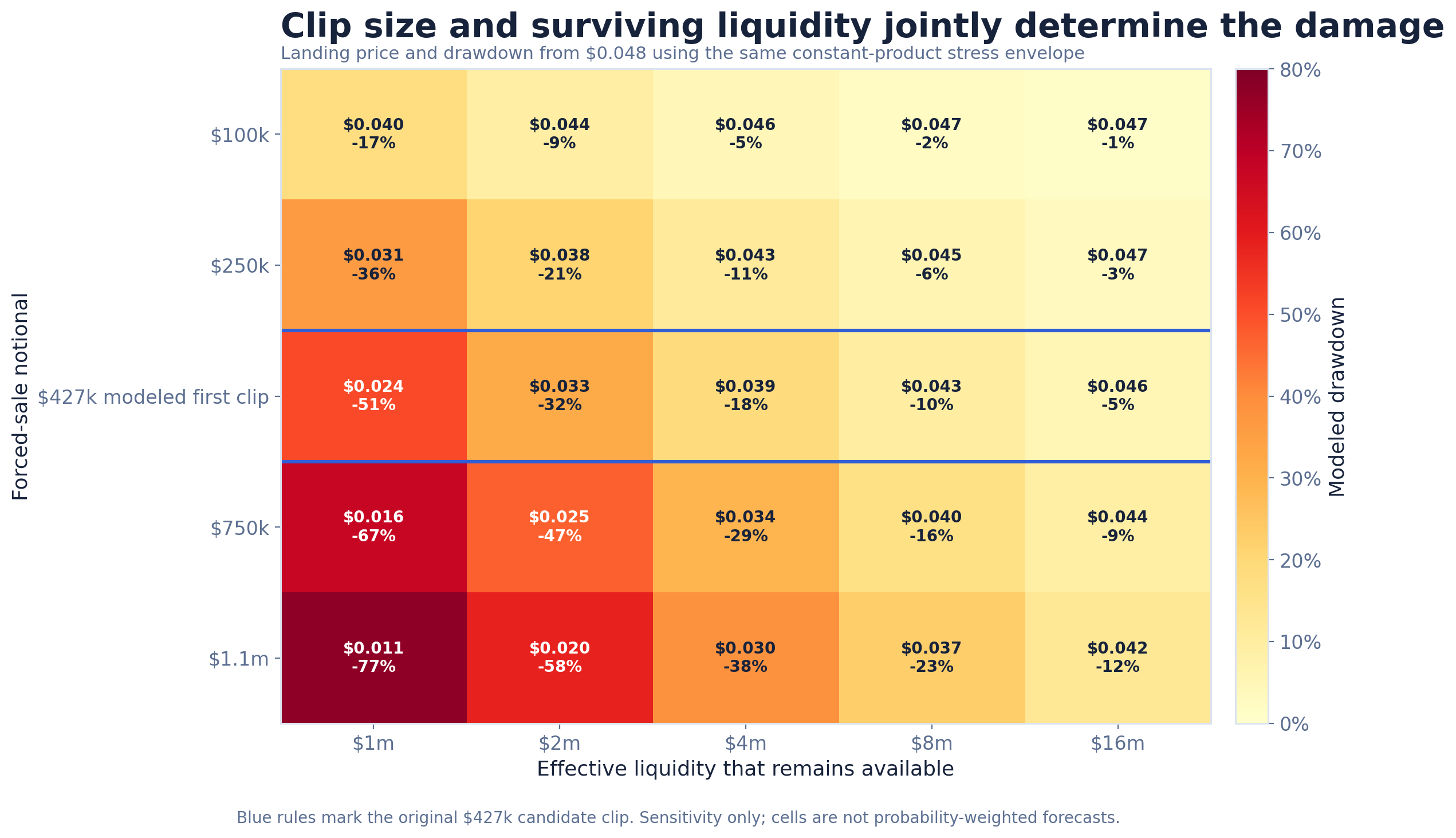
The next issue was liquidation convexity:
S seized = debt repaid * (1 + collateral bonus) / S priceThe same fixed-repayment sensitivity summarized above is plotted across a wider price range here:
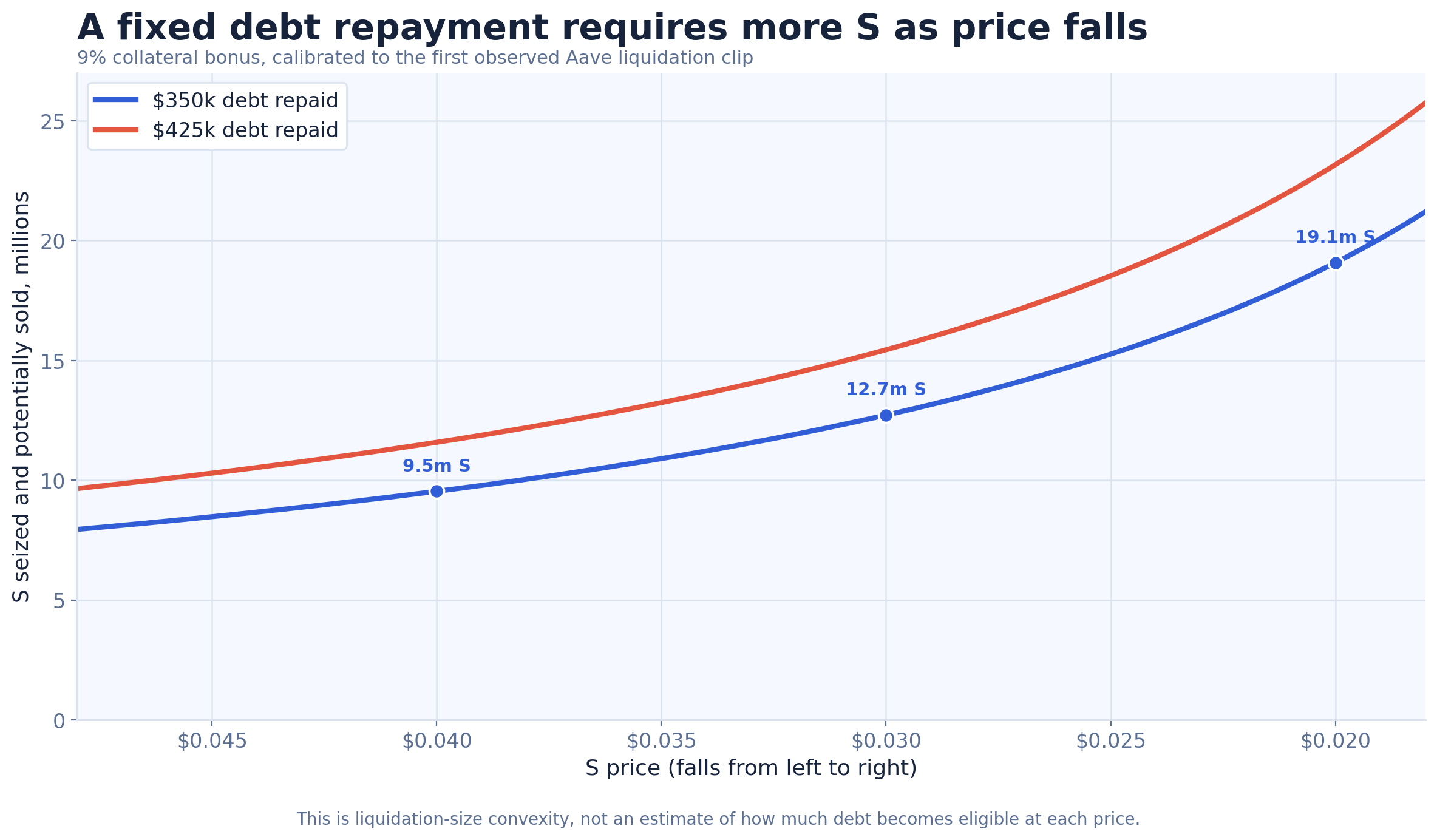
This chart shows how much collateral a fixed repayment requires, not how much debt becomes eligible at each price. A complete second-order supply curve would require a historical account-level snapshot of every S-backed borrower. I tested synthetic borrower buckets during research but excluded them from the reported results because they were not observed positions.
Once expected liquidation loss and withdrawal illiquidity exceeded the remaining carry, I began exiting:
expected residual carry < expected liquidation loss + withdrawal-illiquidity costEngineering The Unwind
USDC liquidity arrived intermittently, often in roughly $25k to $50k clips. I built a Rust event listener and Solidity helper that reacted to those deposits and atomically unwound the cross-protocol loop while maintaining a target health factor.
The listener watched USDC transfers into the Silo over WebSocket and kept a signed EIP-1559 transaction ready, refreshing nonce and fees every five seconds. The contract withdrew safe Silo USDC, repaid Aave USDC, withdrew safe wS from Aave, and repaid Silo wS debt to unlock the next slice.
The bot turned sporadic market liquidity into a controlled exit instead of forcing an all-or-nothing withdrawal.
Unwind architecture
The listener verifies the configured bot identity at startup, prevents duplicate in-flight submissions, and reconnects with bounded exponential backoff. The contract separates bot and owner permissions from an owner-only recovery path and exposes iterative unwind, profit-taking, and final-exit modes.
The Catalyst Disappears
While the final unwind was still in progress, the borrower became active for the first time since February 1. Beginning at 22:13 UTC on May 22, they repaid the original Silo debt in several transactions and split the position across accounts and protocols. The secondary address, 0xbb435a52ec1ed3945a636a8f0058ea3cb1e027e8, held the new Aave position.
The refinancing removed the extreme interest-rate squeeze. Immediately after the sequence, the known Aave account held 72.1m S-equivalent ($3.32m) of collateral against $2.01m of USDC debt, a 1.15 health factor. The original Silo account kept a smaller 17.16m S ($791k) against $454,608 of debt, a derived 1.39 health factor.
I completed the core lending exit by May 25 rather than reversing it. More importantly, I did not immediately short S. The thesis required a specific forced seller to be imminent; after refinancing, that condition no longer held. I kept the monitors running and reallocated the capital.
The Setup Returns
The opportunity reappeared in June for a different reason. The original setup had been driven by compounding debt. The second was driven by falling collateral. As S weakened, the refinanced Aave, Silo, and Flying Tulip positions drifted back toward liquidation.
I rebuilt the thesis against the new state rather than reusing the May model. At 10:23 UTC on June 23, one second before the first reconstructed short fill, the Aave account held 94.2m S-equivalent ($2.30m) of collateral against $1.53m of debt with a 1.05 health factor. The borrower had added roughly 22m S-equivalent of collateral and repaid about $480k of debt since the refinancing; the price fall outran both. Roughly nine hours later the first liquidation executed; two blocks afterward, the account still showed a 0.99 health factor.
I used Hyperliquid because expressing the view through Aave or Silo would have added direct exposure to potential bad debt. Keeping execution on one venue simplified margin, monitoring, and manual risk control.
The plan was to prepare below roughly 1.05 health factor, scale as the account approached 1.00, size against Hyperliquid depth and slippage, and exit if the borrower intervened. Monitoring and position-state calculation were automated; entries remained manual.
Executing The Short
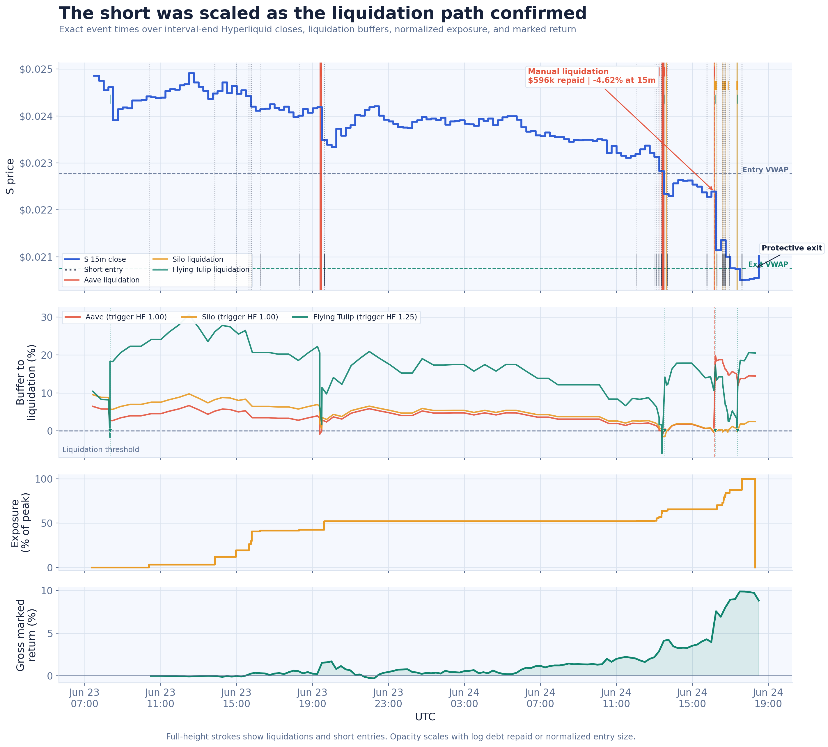
The reconstructed campaign began about nine hours before the first Aave liquidation. I had 42.6% of eventual peak exposure open before that burst, 64.0% before the first Silo liquidation, and 73.3% when my Silo runner later found an eligible liquidation but could not build a profitable DEX route.
The expanded log reconstruction found 662 transaction-level clips during the chart window: 575 on Aave, 83 on Silo, and four on Flying Tulip.
Grouping clips into eight episodes separated by at least five quiet minutes, all eight were followed by a lower completed Hyperliquid candle at the 15-minute horizon. The median move was -2.22%; weighting by debt repaid produced -3.80%. The largest episode began at 16:08 UTC, included the manual Aave liquidation, and was followed by -4.62% at 15 minutes and -6.20% at 30 minutes.
The liquidation timing and subsequent declines were tightly associated. That is consistent with the forced-flow thesis, but it is not a clean causal estimate: falling S triggered the liquidations, and the liquidations could then reinforce the same move.
| Execution measure | Result |
|---|---|
| Holding period | 31h 55m |
| Opening orders / total fills | 32 / 181 |
| Entry / exit VWAP | $0.02277 / $0.02075 |
| 15-minute marked MAE / MFE | -0.30% / +9.90% |
| Fee and funding drag | 16.47 bps of opening notional |
| Gross / net return on opening notional | 8.84% / 8.67% |
| Net PnL / margin transferred for the campaign | 103.6% |
Return on opening notional is the cleanest execution metric, so 8.67% net is the number I quote. Against the margin I actually transferred for the campaign, the same PnL was 103.6%—the opening notional was about twelve times that capital—which measures how hard I sized into the thesis rather than the quality of the trade.
The campaign’s 15-minute position-aware maximum adverse excursion was only 0.30% of final opening notional, which reflects the gradual scaling. The reduce-only stop preserved most of the move but captured 76.9% of the entry-VWAP-to-period-low opportunity, closing about 1.06 percentage points below the best gross marked return.
The thesis and the early staging were right. The trade made money; the late adds and the exit are where I left some on the table.
Execution timeline and reconstruction methodology
| Time UTC | Execution state |
|---|---|
| 2026-06-23 08:20 | First observed Flying Tulip liquidation clip |
| 2026-06-23 10:23 | First short fill, roughly nine hours before the first Aave liquidation |
| Before 2026-06-23 19:23 | 42.6% of eventual peak size was open |
| 2026-06-23 19:23:08 | Aave burst began; 198 clips repaid $141,062 over the episode |
| 14 minutes after the Aave burst began | Position increased as the liquidation sequence matched the modeled path |
| Before 2026-06-24 13:36 | 64.0% was open before the first Silo liquidation |
| 2026-06-24 16:35 | 73.3% was open when the Silo runner found an eligible clip but failed to build a route |
| 2026-06-24 17:36 | Final scale-in completed |
| 2026-06-24 18:18 | Full position closed through a reduce-only stop as S rebounded |
The figure joins public 15-minute S candles to fills reconstructed through Hyperliquid’s public info API. Exposure is normalized to peak so the sequencing is visible without disclosing position size. The marked-return series uses exposure open at each candle close and divides gross marked PnL by final opening notional. Hyperliquid closes are stepped at the end of their 15-minute interval, so an event inside a candle appears before that candle’s completed close rather than midway through an interpolated decline.
Health factors are historical protocol views sampled at Sonic blocks roughly every 24 minutes, with additional pre/post snapshots around liquidation episodes. The plotted values are exact end-of-block reads; the continuous lines use linear visual interpolation between observations and should not be read as continuously observed protocol state or intra-block ordering. Aave uses getUserAccountData; Silo is derived from collateral assets, USDC debt, the historical solvency-oracle quote, and its 80% liquidation threshold; Flying Tulip uses its native userOverview equity-to-maintenance ratio. Aave and Silo liquidate below 1.00. Flying Tulip’s historical configuration made positions eligible below 1.25; 1.50 was the separate safe threshold for user actions. The chart therefore shows percentage buffer to each protocol’s own trigger rather than plotting unlike raw ratios on one axis.
The Flying Tulip below-trigger samples were all followed by observed liquidations. The June 23 sample preceded its clip by one second. The two June 24 samples belonged to the same episode and preceded the next clip by 8m49s and 9m24s. Eligibility did not imply instantaneous execution; the green dotted lines and threshold markers show when the liquidation transactions actually landed.
| Episode start UTC | Protocols | Clips | Debt repaid | S move after 15m | S move after 30m |
|---|---|---|---|---|---|
| Jun 23 08:20 | Flying Tulip | 1 | $10,171 | -2.88% | -1.93% |
| Jun 23 19:23 | Aave | 198 | $141,062 | -2.91% | -3.32% |
| Jun 24 13:15 | Aave | 1 | $4,628 | -2.13% | -2.32% |
| Jun 24 13:23 | Aave, Silo, Flying Tulip | 366 | $195,035 | -2.32% | -1.15% |
| Jun 24 16:08 | Aave, Silo, Flying Tulip | 65 | $689,025 | -4.62% | -6.20% |
| Jun 24 16:35 | Silo | 12 | $22,600 | -1.66% | -2.82% |
| Jun 24 16:52 | Silo | 4 | $10,600 | -1.18% | -1.23% |
| Jun 24 17:20 | Silo, Flying Tulip | 15 | $22,277 | -1.14% | -1.11% |
Episode returns use the last completed candle before the first clip as the reference and the last completed candle available after the episode horizon. The five-minute separation rule prevents a dense run of bot transactions from being misreported as hundreds of independent observations. The eight episodes remain a small, endogenous sample without a market-factor control, so the table describes temporal association rather than standalone price impact.
MAE and MFE are position-aware 15-minute marks, not tick-level extrema. The favorable-move capture describes the observed entry-VWAP-to-campaign-low price path; it does not assume the full position was open throughout.
The 103.6% figure divides realized PnL by the margin capital explicitly transferred for the campaign. It is a narrow denominator—campaign margin, not whole-account equity—so it reads as a sizing measure, and return on notional stays the headline.
Results
| Leg | Holding period | Result |
|---|---|---|
| Levered Silo/Aave carry | 24 days | 21.79% net ROE after marked S borrow cost |
| Hyperliquid short | 31h 55m | 8.67% net on opening notional after fees and funding; 103.6% of the margin transferred |
The percentages should not be added: the carry leg is return on net USDC equity over 24 days, the directional leg is return on opening notional over 31h 55m, and the margin figure is a sizing measure on a campaign-specific denominator. What they share is the process—the yield anomaly found the stressed market, and the public solvency state later found the trade.
The Liquidation Path I Missed
My key model error was treating DEX capacity as the primary limit on liquidation size. That matched the Silo bots I had observed: borrow through a flash loan, repay debt, seize S, sell it on-chain, and repay the loan. It did not describe every possible liquidator.
The first Aave liquidation sequence began at 19:23:08 UTC on June 23 and followed the expected partial-clip path: 198 transactions repaid $141,062 over the episode. One early clip repaid $143.92 for 6,774 S. The first Silo liquidation followed on June 24, repaying $500 and seizing roughly 23,664 S.
Then a manual operator used a route I had not modeled. At 16:09 UTC on June 24, an Aave transaction repaid $596,209 and seized 29,658,154 wS (about $650k at the oracle price). In a public post, the operator said they hedged the seized collateral via Binance.
This bypassed the immediate DEX bottleneck. The liquidator funded the repayment from its balance sheet, warehoused the wS, and hedged the price risk off-chain. The collateral still had to be carried or eventually unwound, but it did not need to hit the spot market inside the liquidation transaction.
The old notebook’s worst-case full DEX cascade did not occur. Liquidations arrived in partial clips, and the largest operator avoided an immediate 29,658,154 S spot sale. The realized path was still violent—every episode above printed lower, and the largest was down 7.36% an hour later—but those are endogenous moves, not causal estimates.
The model correctly identified forced-flow risk, but it modeled only the liquidators I had already seen. A well-capitalized operator could replace DEX capacity with balance sheet and perp liquidity.
Observed model error and revised liquidation constraints
Later that afternoon, my Silo runner showed the contrast:
2026-06-24T16:35:48Z block=74595828
maxLiquidation: collateral=1,209,596 S, debt=24,204 USDC
route build: OpenOcean swap failed
The runner correctly skipped a DEX-dependent liquidation it could not route. The manual Aave operator had already demonstrated another path:
q_total = q_atomic + q_warehoused

q_total <= protocol liquidation allowance
q_atomic <= profitable DEX route capacity
repayment capital(q_warehoused) <= available balance sheet
q_warehoused <= executable off-chain hedge capacity
shared market impact(q_atomic, q_warehoused) <= risk budget| Model claim | Observed event | Assessment |
|---|---|---|
| Liquidation would occur through partial repayments | Aave and Silo both liquidated in clips | Confirmed |
| DEX economics would constrain flash-loan liquidators | The Silo runner found debt but could not build a route | Confirmed |
| Seized collateral needed an immediate DEX sale | The manual operator warehoused the seized wS and hedged via Binance | Incorrect |
| Off-chain liquidity could absorb immediate pressure | The operator used Binance to hedge the seized collateral | More important than modeled |
| Borrower intervention could remove the catalyst | The May refinancing paused the thesis | Confirmed |
The atomic and warehoused routes can compete for the same underlying spot and perp liquidity. The warehoused route also introduces basis, funding, margin, counterparty, and eventual collateral-disposal risk.
Execution Review
| Decision | Assessment | Revised rule |
|---|---|---|
| Scale gradually as health deteriorated | Strong | Retain staged entries tied to borrower and market state |
| Cross the book for every order | Weak | Rest passive entries before the catalyst; take liquidity only when urgency exceeds spread and fee costs |
| Add after the manual liquidation | Weak | Treat every material repayment as a new underwriting decision |
| Hold through the rebound | Acceptable, not optimal | Place reduce-only profit orders across modeled stress levels |
| Exit with a protective stop | Fair | Keep the stop, but use it for residual exposure after taking profit |
The weakest decision was adding after the manual Aave liquidation. I treated the event as confirmation even though it materially reduced the borrower’s debt and avoided the immediate DEX sale I had modeled. Holding the existing short could still make sense, but increasing it required evidence that meaningful forced selling remained.
Instead, the final scale-in completed after the campaign’s best marked-return interval and shortly before the protective exit. I increased risk when the catalyst was most visible but the remaining edge was smallest.
The other clear weakness was execution style. All entries were taker orders even though the campaign began roughly nine hours before the first Aave liquidation. Crossing the spread was defensible once liquidation flow was live and at the protective exit, but early staging did not require the same urgency. Historical fills do not preserve the full order book needed for a reliable passive-execution counterfactual, so I cannot quantify the exact spread savings; the decision rule is still clear.
The research found the trade and gradual scaling controlled the early risk. The next improvement is recognizing when the trade has already worked.
The Catalyst Gets a Calendar
Two months after the June liquidations, the residual position is still the largest constraint on this market—and it has just acquired a schedule. At Sonic block 78080083 on August 24 at 15:20 UTC, Aave reported $1.37m of collateral against $600,094 of USDC debt: a 1.57 health factor against a 69.02% weighted liquidation threshold. The collateral is 24.7m wS plus 21.7m stS—roughly 48m S-equivalent—and the debt is 42.9% of all USDC borrowed on the deployment.
Six days earlier the same account read 1.18. Nothing about the position changed between the reads; S closed August 18 at $0.0214, within about 6% of June’s liquidation-cascade low, then rallied 33% by August 24. A balance sheet this concentrated in one thin asset re-prices its own solvency daily.
The schedule arrived on July 29, when LlamaRisk published an ARFC deprecating Aave’s six lowest-adoption deployments, Sonic the largest among them: deposits had fallen 74% in six months to $7.6m, generating under $5k of quarterly revenue. The Snapshot vote passed unanimously on August 15; as of the August 24 snapshot, no Sonic reserve is frozen yet, so the on-chain execution is still pending. When it lands, every Sonic reserve is frozen with caps reduced to 1—blocking new supply, new borrows, and new collateral—while borrowed reserves like USDC move to a 99% reserve factor and a 5% base rate. The proposal then reserves two explicit escalation levers: steeper rate curves where borrowers do not repay, and stepwise liquidation-threshold reductions to remove lingering collateral positions.
The Squeeze Arithmetic
The base-rate step roughly doubles the account’s current 3.90% USDC borrow cost, but rates alone are a slow clock: at 9%, compounding debt needs about 5.3 years to erode a 1.57 health factor at flat collateral value, and even 50% needs over a year. The threshold ladder is the fast dial. Holding debt and collateral composition constant:
| Liquidation threshold | S decline to eligibility |
|---|---|
| 69.02% (current) | 36.4% |
| 65% | 32.4% |
| 60% | 26.8% |
| 55% | 20.2% |
| 50% | 12.2% |
Governance moves the threshold and the market moves the price; eligibility is wherever they meet. The interaction is violent: flat-price eligibility currently requires stepping the threshold near 44%, but on August 18’s close it sat near 58%—a 33% rally moved the trigger fourteen points in six days. Until the freeze executes, the borrower can still deposit collateral—migrating the 4.76m S (about $136k) they still hold on Silo would lift the health factor toward 1.7—so the pre-execution window is also their cheapest defense.
The June episodes needed a falling market. The wind-down only needs its own playbook: governance steps the threshold down, and the market merely has to stand still.
Every Door Is Smaller Than the Position
Whether the endgame is voluntary repayment or liquidation, both run through the same exits, and I re-measured them on August 24:
| Exit or hedge route | Measured capacity |
|---|---|
| wS to USDC, aggregator-routed, 5m wS clip | $130–131k out, ~8% below spot |
| wS to USDC, aggregator-routed, 24m wS, roughly the account’s wS stack | $212–234k out, 66–69% below spot |
| stS to USDC, aggregator-routed, any size from 5m to 24m | $44–144k out, router-dependent, then saturated |
| stS to S at par via Beets unstaking | 14-day unbonding queue |
| Binance S/USDT bids within 2% of mid | ~$102k |
| Hyperliquid S perp open interest | $740k, funding ~+11% annualized to shorts |
| Silo S/USDC idle USDC, the only other lending venue in this study | $53k |
In May, aggregator routes could still absorb roughly $600k of S before slippage consumed the economics. Today the account’s whole wS stack surrenders $212–234k of USDC, and the stS half of the collateral is the sharper problem: the better-routed quote saturates near $144k, the second router finds under $45k, and both drain the same downstream wS/USDC pools as the wS routes, so the ceilings do not add. Beets’ 14-day unbonding queue remains the only par exit. Repaying $600k by selling collateral is therefore still not executable on-chain at tolerable impact; it means external capital, weeks of queued unstaking and dribbled sales, or a CEX book showing $102k of near-mid bids.
The liquidator’s constraint set re-prices the same way. A first clip at the protocol’s 50% close factor could repay about $300k and seize roughly $330k of collateral at the configured 10% bonus—around 12m S-equivalent, or 1.4–1.6x the total USDC the measured wS routes can produce. Liquidators choose which collateral to seize, so wS goes first and later clips inherit the stS side: an asset with fragmented, router-dependent instant depth and a two-week par exit. That favors, again, the balance-sheet operator who warehouses and hedges. The carry is currently free—positive funding pays shorts about 11% annualized—but a $330k hedge is nearly 45% of all existing S open interest on Hyperliquid, so the hedge itself moves the market it needs. The alternative to an orderly clip sequence is the DAO’s own threshold ladder outrunning liquidator capacity and stranding bad debt on a deployment it is trying to close, which is precisely the outcome the escalation levers are written to avoid.
In May, interest rates manufactured the forced seller. In June, price did. The third act is administrative: the venue itself is scheduled to close, and every measured path out of the position is smaller than the position.
What turns this from analysis into a trade is unchanged from June: proximity to eligibility and evidence of actual forced flow. The monitoring list now starts with the governance calendar—AIP submission, the execution payload, each subsequent threshold step—then the familiar surface: borrower top-ups or repayments before the freeze, S price against the ladder, aggregator route capacity, perp depth and funding, and which of the two liquidator archetypes this study documented shows up first.
Wind-down snapshot methodology and quote provenance
Position state is an atomic read at Sonic block 78080083 (August 24, 2026, 15:20 UTC): getUserAccountData for the account, aToken and variable-debt balances for composition, and the variable-debt token’s total supply for the 42.9% share of deployment USDC borrows. Reserve parameters—liquidation thresholds, the 10% wS/stS liquidation bonus, and the not-yet-frozen flags—are decoded from getReserveData configuration bits at the same snapshot.
The threshold ladder is static arithmetic on that snapshot: it holds debt, collateral quantities, and the wS/stS mix constant and asks what uniform collateral-price decline reaches health factor 1.0 at each hypothetical threshold. The weighted threshold shifts slightly as wS and stS prices move relative to each other, and the escalation levers are proposal language, not executed parameters. The debt clock is pure compounding against flat collateral value. No probabilities are assigned to any row.
Exit quotes are point-in-time responses from the KyberSwap and OpenOcean public quote APIs on August 24 for 5m and 24m clips of wS and stS into native USDC; the ranges span the two routers. The routers disagree on stS by roughly 3x—venue integration is fragmented—so the range is reported rather than averaged. Aggregator quotes depend on integrated venues and routing at that moment and are not firm liquidity. Binance depth sums visible S/USDT bids within 2% of mid from the public order-book endpoint at roughly the same time; order-book depth is ephemeral. Hyperliquid open interest and hourly funding come from its public info API, with funding annualized from the hourly print; funding floats continuously. The Silo figure is the USDC silo’s idle token balance at the snapshot, and the borrower’s residual 4.76m S of Silo collateral is their collateral-share balance converted to assets.
Generalizing The Signal
The core lesson is that on-chain transparency does not mean every visible risk is priced. Collateral, debt, rates, health factors, and DEX liquidity were public. The edge came from joining them into a forward view of who might be forced to trade, when, and through which route.
The process was a chain of public inputs: utilization to find the stress; rate mechanics to project the debt path; wallet behavior to judge whether the borrower would step in; health-factor modeling to locate the trigger window; DEX, CEX, and perp depth to test whether the exits could absorb it; liquidator behavior to correct the model when the realized route differed; and now the governance calendar to catch forced flow that arrives by vote.
That is the process I am now generalizing into a protocol-agnostic system: map public lending positions into potential future orderflow, estimate liquidation eligibility and clip size, test atomic and balance-sheet-funded unwind paths, and compare expected impact against spot and perp liquidity.
This case began with a routine scan of Silo’s small lending markets. It ended as a live example of how public protocol state can reveal future orderflow before it reaches the market.
Written by
Kai Aldag
I build and write about crypto, cryptography, and distributed systems. Egg Tech is my one-person company — the home for what I ship and the notes I keep along the way.